Revised in 2010
7.17.1 Introduction
The main aim of the VG subprogramme is to obtain sensitive bioindication of changes in pollutant deposition or other atmospheric factors, e. g. warming, on a representative plant community and its species. Another aim is to obtain data on the dynamics of tree biomass and canopy structure representative at least for the intensive area where a number of subprogrammes are also being conducted. This is especially important where the BI subprogramme (Tree bioelements and tree indication) is lacking. Data on dead trees, logs and stumps are useful for following the decay process and the dead wood as habitat for fungi, mosses and insects. Also detailed monitoring of soil-living plants as part of the biological diversity of the site is achieved.
The understorey vegetation includes soil-growing vascular plants, bryophytes and lichens, not fungi or algae.
For the interpretation of data it is especially important to have access to data from subprogrammes Precipitation chemistry (PC), Throughfall (TF) and Soil chemistry (SC).
7.17.2 Methods
7.17.2.1 Selection and establishment of the plot
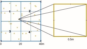
Establish one or two permanent intensive plots about 40x40 m (preferably between 20x20 and 50x50 m) (Fig. 7.17.1) in a homogeneous part of one or two plant communities representative of the monitoring site and preferably also widespread in the region. Establish the plot when most plants are fully developed. It is practical to orientate the plots in north-south/east-west directions. Mark permanently the corners of the plot.
|
|
|
|
|
Figure 7.17.1. An example of an intensive plot (40x40 m). Sample plots (SP, 50x50 cm) for understorey vegetation are distributed in a stratified random fashion - each 10x10 m subsquare (SS) is sampled by, for example, two random plots. The intensive plot can be subdivided into four quarters (Q, 1-4), but this is not obligatory because more subsquares, each with two sample plots, were chosen in some IM sites.
|
Distribute randomly or by stratified random sampling a sufficient number of sample plots, e. g. 50x50 cm, on the intensive plot and mark them permanently (Fig. 7.17.1). In order to counteract unwanted activity from animals on the sample plot the marking should be insignificant. 20-40 plots should be sufficient, depending on the variability of the understorey vegetation and the size chosen of the sample plots. Exclude plots where unwanted substrates, e.g. stone or log occupy more than a certain part. Make sure that disturbing influence, e.g. trampling, especially on the small sample plots, from various monitoring activities are excluded.
7.17.2.2 Observations
According to its stratification and functional groups the vegetation of the intensive plot should be separated into layers. No specific height limits of trees and shrubs can be given, but here is an example:
-
tree layer: trees > 5 m
-
shrub layer: trees 1-5 m, morphological shrubs >1 m
-
field layer: trees and shrubs <1 m, other vascular plants irrespective of height
-
bottom layer: bryophytes and lichens
According to this classification a tree species can be present in both tree, shrub and field layers. If desirable the tree layer could be separated into an upper and a lower stratum.
Tree layer and dead wood
Observe living and dead trees that belong to the tree layer according to definition and, if feasible, also logs and stumps over the whole intensive plot!
- Note the species of all trees and other objects mapped and measured!
- Map the trunk bases of living and dead trees, preferably by coordinates using an origo, e. g. the SW corner of the intensive plot.
- Note dbh (=diameter at breast height, i. e. 1.3 m above ground) (cm) of all trees mapped, crown diameter (m) and crown limit (m) only of living trees. Where the tree crown is very eccentric a diameter value is estimated which gives an approximation of the real cover.
- Measure the heights (m) of trees. Where trees are numerous and tops difficult to see heights could be measured only on a selection of representative individuals of different dbh-classes. Then the heights of the others are estimated using the regression between dbh and height.
- Logs and stumps (clearly not connected with logs) above a minimum size, e.g. 5 or 10 cm diameter, should also be mapped and measured. The position and length of a log can be inferred from co-ordinates for its top and base ends. Dbh should be measured 1.3 m from the base to be comparable with that of standing trees. On tall stumps (1.3 m) dbh is measured, on low ones the diameter of the upper surface.
Take care to avoid trampling on the small sample plots when mapping and measuring the trees and shrubs!
Shrub layer
Map living and dead trees and shrubs in the shrub layer, according to definition, in the same way as trees of the tree layer. Where a shrub has several trunks the thickest is chosen for position and dbh measurement. Thickets of shrubs may be mapped directly by drawing the outline on a map of the intensive plot.
Field and bottom layers
The main parameter observed is quantity, expressed as percentage cover for all individual species. In order to keep external conditions as uniform as possible, only plants living on relatively homogeneous soil should be included. This excludes plants growing on other substrates, e.g. stones and logs.
Estimate the cover of the field and bottom layers and their species. Cover percentage (%) of the sample plot is the area that above-ground living parts of a plant occupy when projected vertically on to the ground (shade when sun in zenith) (Figure 7.17.2). A mesh, made of a frame and strings, with 10x10cm mesh size can be put on sample plots in order to help estimating cover. Do not remove specimens from the sample plots. If identification requires samples for determination they must be sought outside the plots.
| In the 1998 version of the manual vigour expressed as flowering value was also used. The monitoring of this parameter can be continued but its value for bioindication is of minor importance. Subsequently spatial distribution, expressed as plot frequency, is calculated if reporting is done according to the old manual. |
Optional: Vigour
Estimate presence of flowering organs (bud, flower, fruit, fruit rest of the current year) of species in the field layer using the fertility codes:
- 0 = species sterile
- 1 = <10 % of all shoots/individuals with flowering organs
- 2 = >10 % of all shoots/individuals with flowering organs
|
|
|
|
|
Figure 7.17.2. Six cases of plant cover. Test your accuracy of cover estimate! (True values in % after paragraph 7.17.4.)
|
7.17.2.3 Frequency of observations
Tree and shrub layers should be observed every five years.
Depending on the stability and vulnerability of the vegetation, the intervals between observations of the field and bottom layers could be 1 - 5 years. In order for a time-series to be established as soon as possible annual observations are recommended. Make observations when the majority of species are fully developed. In deciduous forest there may be two peaks of development, one before leafing and one later.
7.17.3 Quality assurance/Quality control
As far as possible the same person should do all estimates - as separate from measurements - at one site. A new observer should calibrate him-/herself against the former. In order to get an estimate of the observer error it is recommended to repeat the estimate of at least 10 sample plots and report the variation. The accuracy of the estimate regarding the true cover may be enhanced by training on computer-made pictures with known exact cover (an example is given in Figure 7.17.2) and/or measuring the cover of at least dominant species on photographs of a selection of sample plots with frame visible on the photo.
Statistical power analysis is a useful tool to calculate the number of plots required to detect a certain change in a variable and, conversely, to calculate which change can be detected with a given number of plots. In both cases the analysis must be based on the known variation of the vegetation on the plots.
7.17.4 Data pre-treatment
Trees
Estimate the height of those trees whose heights were not measured in the field by using the regression between dbh and height of those trees which were measured.
At sites where the BI subprogramme is not performed it is recommended to estimate the biomass of the tree stand of the intensive area using the data from the intensive plot. Thereby the procedure and reporting format of the BI subprogramme should be applied.
Cover (COVE)
| In the 1998 version of the manual aggregated mean values of percent cover of species per quarter were reported. The problem with this reporting schema is twofold: 1) many IM sites did not set up their intensive plots according to the proposed design so that sample plots can not be aggregated to quarters; 2) statistical power is lowered when using aggregated values. Thus, with the new 2010 version of the manual only raw data, i.e. percent species cover per sample plot, is reported. |
Net cover (excluding overlap between individuals) of the tree and shrub layers and their species is given as percentage (%) of the whole intensive plot. Cover of shrub thickets, mapped directly in the field, could be measured on the map. Cover of the field and bottom layers and their species is reported for each sample plot (Fig.7.17.1). The sample plots are the basic units of observation and each must be labelled in the field QUARTER! Each sample plot within an intensive plot must have a unique label. The labelling format describes the design of the intensive plot.
In the new the new 2010 coding system QUARTER describes the design of the intensive plot. If the described design with quarters is used, then e.g. sample plot 2 in subsquare 3 of the first quarter is coded as 132 (Q,SS,SP) in QUARTER. If other designs are used, reporting is done for each sampling plot without including information on the inner design of the intensive plot. In such cases QUARTER is used to number each sampling plot of the intensive plot.
Flowering (FERT)
Flowering value for each field layer species is calculated for all sample plots using the formula:
flowering value (%) = 100 x[ ∑(ni * Fi)] / 2N
where
Fi = 1, 2
ni = number of plots with fertility Fi
N = total number of plots with species occurrence
Example: A species is found on 8 sample plots. On 2 plots it is sterile, on 3 plots it has fertility 1 and on 3 plots fertility 2. Then the calculation will be like a). If it has fertility 2 on all plots, i. e. maximal value, it will be like b):
a) 100 x [( 3 x 1 ) + ( 3 x 2 )] / 2 x 8 = 56% b) 100 x [( 0 x 1 ) + ( 8 x 2 )] / 2 x 8 = 100%
Flowering index (FERT_I) for the whole field layer of all sample plots is calculated as the mean of the flowering values of all species.
Plot frequency (FREQ)
Calculate per cent (%) plot frequency of the whole intensive plot for each species in the field and bottom layers by dividing the number of sample plots where the species is present by the total number of plots and multiplying by 100. When reporting is done according to the new format (sample plot wise) than it is not necessary to calculate and report frequencies.
| In the 1998 version of the manual so called “sensitivity indices” were reported. We rename these indices to “Ellenberg indices” to better reflect what they really are. These parameters are optional and only applicable if the proposed design shown in Fig. 7.17.1 is used. In general, indicator analyses using Ellenberg indices will primarily be done centrally by using sample plot data and harmonised Ellenberg values. |
Optional: Ellenberg indices (R and N)
Original indicator values of species (on a 1-9 ordinal scale) (Ellenberg 1991) or regionally modified ones for soil pH (R) and nutrient (N) preferences are used as a basis for calculation of environmental conditions of a plot. If possible, the indicator values should be modified to fit the region if other than central Europe where Ellenberg's values were established.
Ellenberg indices should be calculated for each quarter of an intensive plot using the formulas:
R-index = ∑Pi*Ri
N-index = ∑ Pi*Ni
where Pi = relative cover of the i th species Ri or Ni = indicator value R or N of the i th species
Proceed thus:
Calculate relative cover of all field and bottom layer species, i. e. the cover of each species divided by the sum of the covers of all species which have an indicator value; the sum of all relative cover values will be 1.
Multiply the relative cover value for each species by its R or N indicator value.
Sum the products. The sum gives the Ellenberg index of.
Values for the Figure 7.17.2, per cent (%) cover:
a: Scor hum 20
b: Desc fle 1.3
c: Paris qua 27
d: Oxal ace 32
e: Vacc oxy 19
f: Alnu inc 22
7.17.5 Data reporting
Mandatory parameters
| Parameters |
list |
|
| COVE_T |
IM |
mean cover of layer/species (%) in tree layer for the whole intensive plot or COVE_T1 and COVE_T2 if the tree layer is divided into two layers |
| COVE_S |
IM |
mean cover of layer/species (%) in shrub layer for the whole intensive plot |
| COVE_F |
IM |
cover of layer/species (%) in field layer per sample plot |
| COVE_B |
IM |
cover of layer/species (%) in bottom layer per sample plot |
| NUM_LD |
IM |
number of living trees per 5 or 10 cm dbh class per species and total CLASS: 0=0-4 cm 5=5-9 cm, 10=10-14 cm, 15=15-19 cm etc.), for the whole intensive plot |
| NUM_DD |
IM |
number of dead trees per 5 or 10 cm dbh class per species and total; (classes as NUM_LD), for the whole intensive plot |
| NUM_FD |
IM |
number of fallen trees (logs) per 5 or 10 cm dbh class per species and total (classes as NUM_LD), for the whole intensive plot |
| NUM_LH |
IM |
number of living trees per 1 or 5 m height class per species and total (CLASS: 1=1.3-4m, 5=5-9 m, 10=10-14 m, 15=15-19 m etc.), for the whole intensive plot |
| NUM_LCL |
IM |
number of living trees per 1 m crown-limit class per species and total (CLASS: 0=0-0.9 m, 1=1.0-1.9 m, 2=2.0-2.9 m, 3=3.0-3.9 m etc.) , for the whole intensive plot |
| NUM_LCW |
IM |
number of living trees per 1 m crown-width class per species and total (CLASS: 0=0-0.9 m, 1=1.0-1.9 m, 2=2.0-2.9 m, 3=3.0-3.9 m etc.), for the whole intensive plot |
Optional parameters
| Parameters |
list |
|
| FERT |
IM |
flowering value per field layer species (%) for the whole intensive plot |
| FERT_I |
IM |
flowering index of all field layer species (%) together |
| FREQ |
IM |
plot frequency per field/bottom layer species (%) for the whole intensive plot |
| SENS_R |
IM |
Ellenberg soil acidity index (R) of the community, i. e. all species in field and bottom layers per quarter (1-4) (2 decimals), report QUARTER! |
| SENS_N |
IM |
Ellenberg nutrient index (N) of the community, i. e. all species in field and bottom layers per quarter (1-4) (2 decimals), report QUARTER! |
Example files
VG example Excel file
VG example ASCIIl file
- File identifier states the subprogramme.
- Species are reported as MEDIUM using codes of the Nordic Code Centre (see Annex 6). Single species not found in the code lists may be reported using preliminary codes (see Annex 6), the full scientific name (including taxonomic authors) with the preliminary code needs to be given separately.
- QUARTER is used to specify each sample plot by either giving a consecutive number or by giving quarter (1-4), subsquare (1-4) and sample plot (1, 2, ..., n) as a 3 (or 4)-digit number. For variables reported for the whole intensive plot, QUARTER is left empty. (In the old 1998 reporting format and where required, the quarters of the intensive plot were indicated in a separate column, e.g. QUARTER= 4 means quarter number 4 and was reported with cover values and Ellenberg indices for the field and bottom layer.)
- Sampling year and month are given as YYYYMM.
- Spatial pool (SPOOL) is the number of sample plots or trees/shrubs from where the mean value is derived.
- Report dbh, height and crown-limit classes as CLASS.
- Report which environmental optimum values that are applied, whether Ellenberg´s original values or others!
- Report the definitions of the layers, especially the minimum sizes of trees and shrubs observed!
- Tree and shrub layer data are derived from the whole intensive plot without subdivisions.
- Attach the layer codes T, S, F, B to the parameter values for the tree, shrub, field and bottom layers respectively!
- If two tree layers are reported, use layer codes T1 and T2!
- Values are reported as mean or sum, i. e. status flags X and S respectively. General information on flags is given in Chapter 4.
7.17.6 References
Bråkenhielm, S. & Liu, Q. 1995. Comparison of Field Methods in Vegetation Monitoring. Water, Air and Soil Pollution 79:75-87.
Ellenberg, H., Weber, H. E., D., R. Wirth, V., Werner, W. & Paulissen, D. 1991. Zeigerwerte von Pflanzen in Mitteleuropa. -Scripta Geobotanica 18.